Valuation Techniques (IFRS 13 Fair Value Measurement)

Last updated: 21 July 2023

The three predominant valuation techniques outlined by IFRS 13 are:

• The market approach.
• The cost approach.
• The income approach.

Entities should select a technique, or a combination of techniques, that is most applicable to their situation and for which adequate data is available to measure fair value. To accomplish this, entities should maximise the application of relevant observable inputs and minimise the use of unobservable inputs (IFRS 13.61-63).

Let’s delve deeper.

Market approach

The market approach utilises prices and other relevant data generated by market transactions involving identical or similar assets and liabilities. Valuation techniques based on the market approach frequently use market multiples derived for certain variables. For instance, businesses are commonly valued based on their revenue or EBITDA multiples. Matrix pricing is another method mentioned by IFRS 13, whereby the fair value of specific financial instruments (usually bonds) is measured by interpolating values for similar instruments (for instance, similar credit rating of the issuer, maturity, etc.) arranged in a matrix format (IFRS 13.B5-B7).

The market approach is commonly used for measuring:

• Cash generating units and businesses (by referencing quoted prices or transactions within the same industry and based on revenue, EBITDA, or other multiples).
• Properties (by referencing transactions for similar properties).

--

Overwhelmed by constant stream of IFRS updates? Too many newsletters that you move to ‘read later’ folder, but later never comes? Reporting Period has you covered! All essential IFRS developments and Big 4 insights in one place. Carefully curated by Marek Muc and delivered to your inbox monthly. 100% free, no spam, unsubscribe anytime.

Cost approach

Often referred to as the current replacement cost, the cost approach aims to represent the sum that would presently be required to replace the service capacity of an asset, adjusted for obsolescence (for example, physical deterioration, technological or economic obsolescence). This valuation technique assumes that a market participant wouldn’t pay more for an asset than the cost for which it could acquire the service capacity of that asset elsewhere.

The cost approach is typically used for the measurement of:

• Tangible assets that have been internally developed.
• Assets that are utilised in conjunction with other assets and liabilities (IFRS 13.B8-B9).

Example: Current replacement cost of specialised equipment

On 1 January 20X1, Entity A purchased a specialised piece of equipment for $1 million. On 31 December 20X4, Entity A was acquired by Entity X, which must recognise this equipment at fair value under IFRS 3 requirements. The equipment was heavily customised to meet the needs of Entity A and there isn’t identical or similar equipment readily available on the market. To resolve this issue, Entity X obtains price lists of equipment similar to that held by Entity A at 1 January 20X1 and 31 December 20X4 and determines that the prices have risen by 20% during that period. Entity X establishes that this is a reasonable approximation of a price increase that would have to be paid to acquire the customised equipment held by Entity A. Consequently, the replacement cost of a new piece of identical equipment is determined to be $1.2 million. However, this isn’t equal to the fair value as at 31 December 20X4, as it needs to be adjusted for obsolescence. Field experts working at Entity A determined that the equipment should be valued at 70% of the new equivalent. Therefore, the fair value is determined to be $0.84 million ($1.2 m x 70%).

---

Income approach

The income approach converts future amounts (such as cash flows or income and expenses) into a singular discounted amount, taking into account various factors, including risk and uncertainty (refer to IFRS 13.B15-B17). When utilising the income approach, the fair value measurement mirrors the current market expectations about those future figures. IFRS 13 provides examples of valuation techniques that align with the income approach, including present value techniques, option pricing models, and the multi-period excess earnings method (IFRS 13.B10-B11).

Present value techniques

Paragraphs IFRS 13.B12-B30 provide comprehensive guidance on the application of present value techniques. The focus is predominantly on the discount rate adjustment technique and the expected cash flow technique, but this does not limit the usage of other techniques (IFRS 13.B12). Generally, present value techniques discount estimated future cash flows to a present amount using a suitable discount rate. IFRS 13.B13 highlights elements that a present value technique should incorporate, whereas the general principles can be found in IFRS 13.B14.

Present value techniques are commonly used for the measurement of:

• Cash-generating units and businesses (based on projected revenue and expenses).
• Financial assets and liabilities when quoted prices are not available for identical or similar items (based on contractual and/or estimated cash flows).
• Investment properties (based on projected rental revenue and operating expenses).

Discount rate adjustment technique

The discount rate adjustment technique employs a singular set of cash flows from the range of possible estimated amounts, be they contractual or most likely cash flows. These cash flows are then discounted using an observed or estimated market rate of return (WACC is most frequently used). Therefore, all risk is reflected in the discount rate. More details and a simple example are provided in IFRS 13.B18-B22. The discount rate adjustment technique is used much more extensively than the expected present value technique discussed below.

Expected present value technique

The expected present value technique is based on an expected value that is commonly used in statistics. It commences with several possible future cash flows with assigned probabilities that result in a singular probability-weighted average amount. Further discussion can be found in IFRS 13.B23-B24.

IFRS 13 differentiates between two methods of executing the expected value technique (refer to IFRS 13.B25-B30). However, I believe this distinction is unnecessary, and I struggle to envisage Method 1 being frequently used in practice. Therefore, when this website refers to the expected present value technique, it refers to Method 2 as outlined by IFRS 13.

Discount rate adjustment technique vs expected present value technique

The discount rate adjustment technique and the expected cash flow technique differ in their risk adjustment and in the type of cash flows they employ. More information can be found in IFRS 13.B15-B17. This difference is illustrated in the example below.

Example: Difference between discount rate adjustment technique and expected present value technique

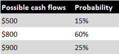
Suppose the expectations about cash flows from a financial asset in one year are as shown below, the risk-free interest rate is 5%, and the market risk premium is 3% (IFRS 13.B27):

The fair value measurement using both techniques is as follows:

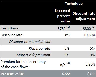
1. Probability-weighted cash flows.
2. Most likely cash flows.
3. Already incorporated in the probability-weighted cash flows.

---

Multi-period excess earnings method

The multi-period excess earnings method is used to measure the fair value of an intangible asset. This valuation technique specifically accounts for the contribution of any complementary assets and associated liabilities in the group in which the intangible asset would be utilised (IFRS 13.B3(d); B11(c)). There are some indirect references to this method in the basis for conclusions to IFRS 3 (IFRS 3.BC177), where it is described as a valuation technique necessitating ‘a contributory asset charge’ to isolate the cash flows generated by the intangible asset being valued from those contributed by other assets. The contributory asset charges are depicted as hypothetical ‘rental’ charges for the use of those other contributing assets.

The multi-period excess earnings method is typically employed to measure intangible assets that other entities cannot readily acquire, such as customer base (see the example below).

Example: Valuation of a customer base and customer relationship using multi-period excess earnings method

On 1 January 20X1, Entity AC, a company providing cable TV services to its customers, acquires Entity TC – one of its local competitors. TC had 100,000 customers at the acquisition date. The acquisition accounting requires AC to recognise the acquired customer base separately from goodwill at fair value. Therefore, AC prepared a valuation using the multi-period excess earnings method, which is presented below. It is highly recommended to view the calculations in an Excel file available for download.

Cash flow projections for the customer base and customer relationship are as follows:

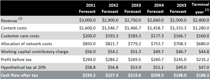
1. The terminal year represents cash flow projections beyond the period covered by the forecast. Typically, it aligns closely with the last year covered by the forecast.
2. Revenue is declining as customers switch to competitors; no new customers are considered in this valuation, as it pertains only to the customer base at the acquisition date.

Other inputs to the valuation are:

• Post-tax discount rate at 7% (e.g., WACC).
• Perpetuity Growth Rate (PGR) at -4.36% – the estimated growth rate beyond the period covered by cash flow projections. For a customer base, this will always be negative (see the second footnote under the table above).

The calculation yields a total fair value of $2,231 million, divided as follows:

• $924 million: present value of cash flows for years 20X1 to 20X5
• $1,307 million: present value of the terminal year.

---

Relief from royalty method

The relief from royalty method is employed for the valuation of assets that are subject to licensing, such as brands or patents. With this method, the fair value of such an asset is calculated as the present value of royalties that would need to be paid to a hypothetical owner of the patent or brand.

Inputs to valuation techniques

Valuation techniques employed to determine fair value should primarily utilise relevant observable inputs, and the use of unobservable inputs should be minimised (IFRS 13.67). These inputs must align with the characteristics of the item being measured, which market participants would consider in a transaction for that item. If no quoted price is accessible, adjustments to the valuation technique might be required to mirror the attributes of the item being measured (IFRS 13.69). Examples of markets where inputs could be observable include foreign exchange markets, dealer markets, brokered markets and, less frequently, principal-to-principal markets (IFRS 13.B34).

Premiums or discounts

Premiums or discounts may be considered in fair value measurement, provided they align with the unit of account and would be factored in by market participants. For instance, a control premium for a controlling stake in an unlisted subsidiary can be considered. This means the fair value of an investment in a subsidiary surpasses the fair value of individual assets and liabilities (IFRS 13.69). However, there’s a specific ‘PxQ‘ rule for subsidiaries listed in an active market.

Premiums or discounts that reflect the size of the entity’s holding rather than an attribute of the asset or liability being measured are not permitted in the fair value calculation. Notably, blockage factors, which are adjustments to the quoted price of an asset or a liability to reflect the fact that the market’s normal daily trading volume cannot absorb the quantity of instruments held by the entity, are not allowed (IFRS 13.69;80).

Bid and ask prices

In the case of an asset or a liability measured at fair value with a bid and an ask price, IFRS 13.70-71 allows for the use of:

• Prices within the bid-ask spread.
• Bid prices for assets and ask prices for liabilities.
• Mid-market pricing or other pricing conventions utilised by market participants.

Calibration

When a fair value at initial recognition matches the transaction price and subsequent fair valuation employs unobservable inputs, the valuation technique must be calibrated so that the outcome of the technique matches the transaction price at initial recognition. This process validates the valuation technique, as further discussed in IFRS 13.64.

Changes to valuation techniques

The valuation techniques used to measure fair value of an item should be consistently applied. A modification in a valuation technique or its application is permitted if it yields a measurement that is equally or more representative of the fair value under the circumstances. IFRS 13.65 provides examples of events that may justify a change in a valuation technique or its application.

A change in a valuation technique or its application is accounted for as a change in an accounting estimate, i.e., prospectively (IFRS 13.66). Nevertheless, IAS 8 disclosures do not apply as IFRS 13 has its own disclosure requirements in this regard (IFRS 13.93(d)).

Use of multiple valuation techniques

IFRS 13.63 acknowledges that there will be instances where multiple valuation techniques will be suitable to measure fair value. In such cases, different valuation techniques will likely yield different results, and the fair value measurement should be the point within that range that most accurately represents the fair value under the circumstances. A wide range of fair value measurements may suggest that further analysis is required (IFRS 13.B40). Examples 4 and 5 accompanying IFRS 13 demonstrate the use of multiple valuation techniques.

International valuation standards

The International Valuation Standards Council (IVSC), an independent organisation, publishes the International Valuation Standards (IVS). These standards can be employed as best practices when preparing a valuation. They are increasingly gaining popularity and recognition among valuation experts.

More about fair value

See other pages relating to fair value: